The previous laboratory script helped you get going with adding
functionality to sxcv.py. The routines you will have added
while doing that script were all simple ones, little more than calls to
single OpenCV routines. This script will go a little further, getting
you to calculate and display histograms of images, then use them to
segment an image. This leads into a look at colour in the next
laboratory.
If you're to figure out how to compute a histogram, the first thing
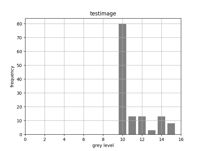
to know is what one is. The graph below shows an example one, computed
for the image produced by the testimage1 routine in
sxcv.py:
im = sxcv.testimage1 ()
x, y = sxcv.histogram (im)
sxcv.plot_histogram (x, y, 'testimage')
(You won't be able to run this code yet as you have to write the
histogram routine.)
The x-axis (the abscissa) plots all the possible grey-level values that a pixel can have, while the y-axis (the ordinate) gives the count of how many pixels of each grey level were found for the image in question. Note that there are no pixels having a value less than 10 in this histogram, and that some 80 pixels have the value 10.
For a colour image, we could compute a single histogram for all
colour bands; but it is generally more useful if we have separate
histograms for each band as shown below for sx.jpg:
im = cv2.imread (sys.argv[1])
x, y = sxcv.histogram (im)
sxcv.plot_histogram (x, y, sys.argv[1])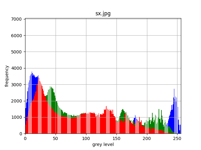
How do you interpret this histogram? Firstly, there are quite a few dark blue and light blue pixels values in the image. The light blue ones are most likely from the pale blue sky, while the dark blue values are probably from the grey values in the building and the rather muddy-coloured water: remember that a grey has red, green and blue components of roughly the same value. The green is most likely from the grass. However, you might be quite surprised by the number of pixels that have a red component, even though nothing in the image appears red. This will again be the red contributions to greyish-looking regions.
You might also ask why there are regularly-spaced comb-like regions in the histogram. These are an aliasing artefact caused by the width of the columns being one grey level wide but the width of the plot on the screen having a number of pixels that isn't a multiple of this value. We shall come back to this at the end of this script.
You don't have a ready-made histogram routine in
sxv.py, so you will have to write one. As with the routines
discussed in the previous laboratory, the starting point is the
documentation and tests:
def histogram (im):
    """
    Return a histogram (frequency for each grey level) of the image `im`.
    The maximum pixel value is determined from the image this is use to
    determine the number of grey levels in the plot.

    The first value returned is an array of the grey levels.
    For a monochrome image, the second value returned is a single-index
    array containing the counts for each grey level; but for a colour
    image, it is a two-index array, with the first index selecting the
    channel (colour band) and the second the counts for that band's
    pixel values.

    Args:
        im (image): image for which the histogram is to be produced

    Returns:
        x (int): grey-level values for the abscissa (x) axis
        y (int): frequency counts for the ordinate (y) axis

    Tests:
        >>> im = testimage1 ()
        >>> x, y = histogram (im)
        >>> print (x)
        [ 0  1  2  3  4  5  6  7  8  9 10 11 12 13 14 15]
        >>> print (y)
        [ 0  0  0  0  0  0  0  0  0  0 80 13 13  3 13  8]

    """
Rather than get you to implement the entire routine from scratch, we shall here look at some parts of it which you need to combine to produce something that works.
You will see from the above code that histogram is
passed in an image and returns two arrays, x giving the
grey level values that appear along the abscissa and y the
corresponding frequencies.
Let us decide that the lowest value plotted on the abscissa will
always be zero. We can find the largest value using the routine
highest which you wrote for the first laboratory, and use
that to set up the values for the abscissa:
levels = highest (im) + 1
vals = numpy.zeros (levels, dtype=int)
for i in range (0, levels):
    vals[i] = i
You might ask yourself why levels is one more than the
value returned by higher --- ask a demonstrator why if you
are unsure. The call to numpy.zeros creates a
one-dimensional array of length levels which will hold
integer values.
If you look at the describe routine, you will see how to
tell whether an image is monochrome (one-channel) or contains multiple
channels. For a histogram, we need code something like
if len (im.shape) == 2:
    # It's a monochrome image, so we have only one histogram.
    ny, nx = im.shape
    hist = numpy.zeros (levels, dtype=int)

else:
    # It's a multi-channel image, so we have a separate histogram for
    # each of its channels.
    ny, nx, nc = im.shape
    hist = numpy.zeros ((nc,levels), dtype=int)
You will see that the monochrome case sets up a one-dimensional array to hold the frequency counts but the multi-channel case sets up a two-dimensional one which you can think of as an array of histograms, one for each image channel.
To compute the actual histogram, we need to iterate over all the
pixels in the image and, for each of them, pull out the grey level value
and add one to the relevant element of the hist array. The
code for the monochrome case is something like
    for y in range (0, ny):
        for x in range (0, nx):
            v = im[y,x]
            hist[v] += 1
and the colour case is somewhat analogous.
This gives you enough information to write the complete
histogram routine, though it requires a little more effort
than just cutting and pasting the code. You will see that the template
in sxcv.py already has a suitable test, so you can check
whether you have it right simply by running the doctests as described in
the first script. The plot-histogram routine is provided,
so once you have it working, you should be able to reproduce the plots
shown in this script.
You will find three images whose names start with
2006-10-23-. Look at the histogram of each image to see how
it tells you whether the image is under-exposed, over-exposed or
well-exposed. This is one reason why most cameras for photography
enthusiasts are able to plot histograms.
Use review.py from the first script on the image
m51.png:
python review.py m51.png
m51.png has 3 channels of size 510 rows x 320 columns with uint8 pixels.
If you are working in the Unix world, you should be able to display
this image using the wonderful xv program:
xv m51.pngIf you type the i key in the xv window, you
will see that it reports the image as 320 x 510 pixels, the same values
as review.py. The displayed image appears black but if you
bring up xv's colour editor by hitting the e
key and then click the button called Random, you will see
that the image suddenly displays many colours. Something weird is
clearly going on.
The cause of the weirdness is that m51.png has 16
bits/pixel, while OpenCV's imread expects there to be 8
bits/pixel by default; that's why it was reported as having
uint8 pixels. This is a good example of OpenCV
doing the wrong thing: it should read the image as a 16-bit
one, or output some kind of warning, or throw an exception --- relying
on the programmer or user to realize what is going on is poor library
design. The solution to this particular problem is to tell
imread that it can read non-8-bit images:
im = cv2.imread (sys.argv[1], cv2.IMREAD_ANYDEPTH)However, this call doesn't work correctly for 8-bit colour images --- it seems that you have to know how the image you are reading is stored on disk, a real annoyance. I am sad to report that there are also many other gotchas with OpenCV that will bite you from time to time.
An 8-bit image has \(2^8=256\) possible grey level values, so a 16-bit one has \(2^{16}=65536\) --- certainly far too many to consider plotting on a histogram because it would be vastly wider than any computer monitor! In fact, even 256 bins is really too many: you can normally glean as much useful information from a histogram having only 64 bins.
Have a go at writing a routine
def better_histogram (im, bins=64):which accepts the number of bins to be plotted as an argument as well
as the image. You can either keep the same behaviour as
histogram and make the lower limit zero, or find both the
lower and upper limits and set up bins equally-sized bins
between these two values. To help implement it, look at section 3.5 of
the lecture notes --- and be sure to include a doctest in your routine
to check that it works. Note that numpy's own histogram
routine also allows you to specify the number of bins.
Although histograms can be useful in their own right to vision developers as well as photographers, they are more often a means to an end as they can be used to perform segmentation, the separation of objects of interest from the surrounding background.
Plot the histogram of the image fruit.png. You will see
that it shows two distinct peaks, one due to the dark-shaded pixels in
the background and the other from the lighter ones in the foreground.
The fruit shows quite a few different grey values because it is roughly
spherical. You can set a threshold to distinguish the pixels in
these two regions: any below the threshold will be deemed background and
any above it foreground. It is useful for subsequent stages of a
complete vision system if all the background pixels are set to zero and
all the foreground ones to 255, giving a binarized image which
identifies these two regions.
We can do the thresholding and binarization by a single OpenCV call
t, bim = cv2.threshold (im, threshold, 255, cv2.THRESH_BINARY)where threshold is the threshold value you have chosen
to separate foreground from background. This returns two values:
t is the value of threshold and
bim the binarized image.
Note that some vision tasks have objects of interest appearing darker than the background. In those cases, we do the thresholding in the same way but flip the meaning of light and dark regions. We shall see an example of this later in the script.
We are using cv2.threshold above in its simplest way: by
changing the last argument in the call, it can be made to do adaptive
thresholding or even compute a good threshold value itself (which is why
it returns t). Your lecturer's view is that this is another
example of bad library design: it would be easier to use if the
different types of thresholding were provided by different routines.
Let us introduce this functionality into sxcv.py as:
def binarize (im, threshold, below=0, above=255):
"""Threshold monochrome image `im` at value `thresh`, setting pixels
with value below `thresh` to `below` and those with larger values to
`above`.  The resulting image is returned.

Args:
    im (image): image to be thresholded and binarized
    thresh (float): threshold value
    below (float): value to which pixels lower than `thresh` are set
    above (float): value to which pixels greater than `thresh` are set

Returns:
    bim (image): binarized image

Tests:
    >>> im = testimage1 ()
    >>> bim = binarize (im, 12, 7, 25)
    >>> print (bim.dtype)
    uint8
    >>> print (bim)
    [[ 7  7  7  7  7  7  7  7  7  7]
     [ 7  7  7  7  7  7  7  7  7  7]
     [ 7  7 25 25  7  7  7  7 25  7]
     [ 7  7 25 25  7  7  7  7  7  7]
     [ 7  7 25 25  7  7  7  7  7  7]
     [ 7  7  7  7 25 25  7  7  7  7]
     [ 7  7  7  7 25 25  7 25  7  7]
     [ 7  7  7  7  7 25  7 25 25  7]
     [ 7 25 25  7  7  7  7 25  7  7]
     [ 7 25 25  7  7  7 25 25  7  7]
     [ 7 25 25  7  7  7  7  7  7  7]
     [ 7  7  7  7  7  7  7  7  7  7]
     [ 7  7  7  7  7  7  7  7  7  7]]
"""
This should call the OpenCV thresholding routine as indicated above,
then set all pixels with values below the threshold to
below and all those above it to above. This
gives the programmer a consistent way of handling situations in which
the foreground is lighter or darker than the background. Note that this
is tricky to get right: you may need a hand from a demonstrator to get
the functionality exactly as specified above.
It will most likely save you some pain in the future if you check
whether the image passed in to your binarize function is a
single-channel one, generating an error message and either exiting if it
isn't or converting it into a single-channel one: there was an OpenCV
call to do this in the previous lab script.
Write a short program to read in fruit.png, threshold
it, and display the segmented image. Experiment with some different
values of threshold, chosen by reviewing its histogram to
identify where it segments best.
Later lab scripts will lead you through using the binarized image to perform the classification of objects.
As a footnote, it is surprisingly difficult to get this binarization
code absolutely correct. You will have seen that
cv2.threshold always sets values below its threshold to
zero, so if above is zero, my own implementation of
binarize wouldn't work --- I should have tested for this
when I wrote the routine but didn't. Here is a test that tripped the bug
in my code:
    >>> im = testimage1 ()
    >>> bim = binarize (im, 12, 255, 0)
    >>> print (bim)
    [[255 255 255 255 255 255 255 255 255 255]
     [255 255 255 255 255 255 255 255 255 255]
     [255 255   0   0 255 255 255 255   0 255]
     [255 255   0   0 255 255 255 255 255 255]
     [255 255   0   0 255 255 255 255 255 255]
     [255 255 255 255   0   0 255 255 255 255]
     [255 255 255 255   0   0 255   0 255 255]
     [255 255 255 255 255   0 255   0   0 255]
     [255   0   0 255 255 255 255   0 255 255]
     [255   0   0 255 255 255   0   0 255 255]
     [255   0   0 255 255 255 255 255 255 255]
     [255 255 255 255 255 255 255 255 255 255]
     [255 255 255 255 255 255 255 255 255 255]]
If you are picky about your code being absolutely correct, do have a
go at making your binarize routine also pass this test.
This approach of:
is known as regression testing. When I worked in industry, we had a test team whose job was to find holes in the code being produced by developers and regression testing was the way in which they did it. It's the best way I know of making your code absolutely correct.
| Web page maintained by Adrian F. Clark using Emacs, the One True Editor ;-) |