Most images are colour, so it makes sense to take a good look at their properties and how to process them. We shall do that in this laboratory script, ending up with segmenting images by colour rather than grey value.
As discussed in lectures, everyone thinks of a colour image as being a combination of red, green and blue channels or bands. You might reasonably expect a colour image to have channel 0 storing red, channel 1 storing green and channel 2 storing blue, and that is the case everywhere except in OpenCV. For some unknown reason (though I suspect it is alphabetical order), the developers chose to order the channels blue, green, red.
| channel | OpenCV | everywhere else |
|---|---|---|
| 0 | blue | red |
| 1 | green | green |
| 2 | red | blue |
With apologies to anyone who suffers from colour blindness, it is easy to confirm this. The following short program sets each channel of an image to be "turned on" in turn and displays the result. If you type in and run this, you will see that the order matches that in the table above. Note that the window name shows which channel is being displayed.
#!/usr/bin/env python
import sxcv, cv2, numpy

ny, nx, nc = 480, 640, 3

for c in range (0, nc):
    im = numpy.zeros ((ny, nx, nc))
    im[:,:,c] = 255
    sxcv.display (im, title="Channel %d" % c, delay=2000)
Take a close look at this code and make sure you understand how all the pixels in a particular channel are being set to 255 --- you will see, and hopefully use, this yourself in later laboratories.
OpenCV provides extensive functionality for converting between colour representations; we shall explore some of these shortly. Before doing that however, it is worth seeing how a monochrome ("grey-scale", "black and white") image is produced from a colour one:
mono_im = cv2.cvtColor (im, cv2.COLOR_BGR2GRAY)Note the American spelling of color and gray; in the UK, we would normally use colour and grey.
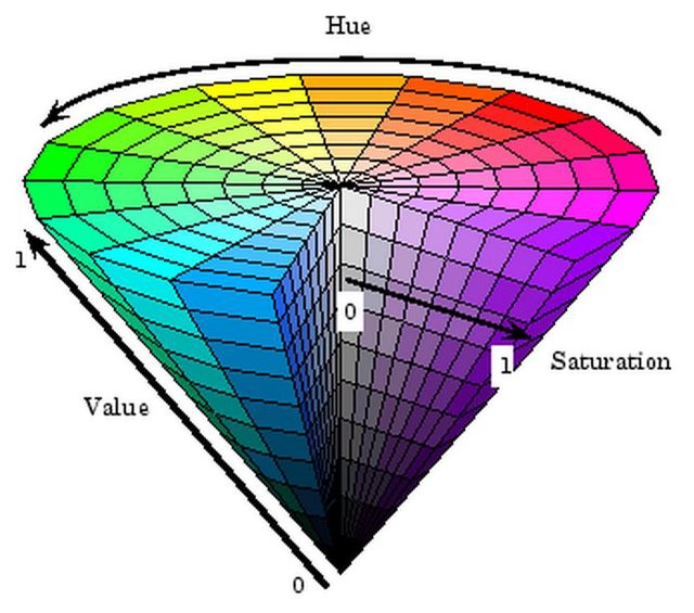
For many computer vision tasks, there are better representations for colour than RGB (or BGR). The most popular is HSV, for hue, saturation and value: see below for what these mean. (The figure is taken from a paper on the web.)

Most people represent hue as an angle measured in degrees and so lying in the range 0 to 360. A mid red is zero degrees, so some shades of red have hue angles above 330 degrees. Both saturation and value are usually given as percentages. OpenCV (you've guessed it) does it differently because it wants the HSV quantities to fit into three unsigned bytes, just as RGB values do. For that reason:
hue is a number in the range zero to 180 (i.e., half the value we normally use)
saturation lies in the range zero to 255, 2.55 times the percentage value
value also lies in the range zero to 255, again 2.55 times the percentage value
Converting sensible HSV values into the OpenCV representation is a
common requirement, so it makes sense to write a routine for
sxcv.py to do that. Paste in the following code and extend
it to do the conversion as outlined above.
def hsv_to_cv2 (h, s, v):
    """Convert HSV values to the representation used in OpenCV, returning the
    result as a tuple for use in cv2.inRange.

    Args:
        h (float): hue angle in the range zero to 360 degrees
        s (float): saturation percentage
        v (float): value percentage

    Returns:
        hsv (tuple): a tuple of values for use with cv2.inRange

    Tests:
        >>> hsv_to_cv2 (360, 100, 100)
        (180, 255, 255)
    """
As before, running the doctests as described in the
first laboratory script will tell you if your code is right.
There is a really good routine in OpenCV to perform segmentation on the basis of colour:
bim = cv2.inRange (im, lo_colour, hi_colour)Here, im is the image to be segmented and
bim the result of the segmentation. lo_colour
and hi-colour are three-element tuples of the lowest and
highest colours of the foreground. Background pixels are represented as
zero in bim and foreground ones as 255. Let us see how to
use it in practice.
The image map.jpg is an image of a map placed on a dark
blue table, part of a system developed in a museum for visitors to set
up the view of a virtual reality reconstruction of medieval London. A
green arrowhead is printed on the image to show the direction of north,
and visitors place the red arrow on it to choose the location and
direction of their view of the virtual environment. Let us concentrate
on identifying the location of the green arrow first.
We are going to do segmentation in HSV colour space. We know that the
colours are cyclic, so both 0 degrees and 360 degrees represent a red
hue. From the diagram above, it is reasonable to conclude that the hue
of green is about 120 degrees and blue 240 degrees. However, how can you
determine them from a real image? In the Unix world (Linx, macOS), the
most convenient way is to use the venerable xv image
display program. This is installed on our Software Lab machines and
Horizon (you should be able simply to make a copy of it if you're
running Ubuntu Linux), while Mac users can ask me for a copy or download and build it.
Simply display the image
xv map.jpgand press the middle mouse button to see the RGB and HSV values of the pixel under the cursor displayed at the edge of the image window. Of course, other programs provide the same functionality, though rarely so easy to access.
As green is about 120 degrees and the arrow is a bright, saturated
shade, we should be able to segment it from map.jpg with
code along the lines of
im = cv2.imread ("map.jpg")
hsv_im = cv2.cvtColor (im, cv2.COLOR_BGR2HSV)
lo_green = sxcv.hsv_to_cv2 ( 80,  50,  50)
hi_green = sxcv.hsv_to_cv2 (140, 100, 100)
mask = cv2.inRange (hsv_im, lo_green, hi_green)
sxcv.display (mask)
As mentioned above, the mask image contains values
similar to the segmentations produced in the previous laboratory script: zero for
pixels in the background and 255 for those in the foreground.
Segmenting red is more difficult than other colours because red spans
both values just above zero degrees and values just below 360 degrees.
However, if you segment both these regions separately and add the
resulting masks together, you should end up with a single mask that
identifies all reds. Try adapting the above code to identify the red
arrowhead in map.jpg.
A little more taxing is segmenting the map region in
map.jpg from the background. The obvious approach is to
convert it to grey-scale and use grey-level thresholding --- but that
doesn't work well because the lines on the map end up as part of the
background too. A better approach in this case is to identify the dark
blue region surrounding the map by colour, resulting in a mask which is
255 for background pixels and zero for foreground ones. This is exactly
the opposite of what is wanted; but as zero has all bits of a byte set
to zero and 255 has them all set to unity, the call
mask = cv2.bitwise_not (mask)flips foreground and background regions. Have a go at this.
The last two paragraphs show some shortcomings in
cv2.inRange for use on real-world tasks, so have a go at
writing a colour_binarize routine that overcomes them. It
should allow the caller to specify the foreground and background values
and make a better job of segmenting red regions.
def colour_binarize (im, low, high, below=0, above=255, hsv=True):
    """Segment colour image `im` into foreground (with value `fg`) and
    background (with value `bg`) by colour.  `low` and `high` are lists
    giving respectively the lower and upper bounds of a 'slice' of
    colours to use for segmentation.  These should be in the same colour
    space as `im`.  The resulting image is returned.

    If `hsv` is set, the colour limits are expected to be provided in
    HSV colour space and so are converted from sensible values into
    those expected by OpenCV by routine `hsv_to_cv2` before use.

    Moreover, if the hue value in the `low` is larger than that in
    `high`, then the hue is taken to span 360 degrees -- this is useful
    when segmenting red regions.

    Args:
        im (image): colour image to be thresholded and binarized
        low (list of 3 values): the lower colour bounds
        high (list of 3 values): the upper colour bounds
        below (float): value to which pixels lower than `thresh` are set
                    (default: 0)
        above (float): value to which pixels greater than `thresh` are set
                    (default: 255)
        hsv (bool): indicates whether `low` and `high` are in HSV space
                    (default: True)

    Returns:
        bim (image): binarized image

    Tests:
        >>> import numpy
        >>> im = numpy.zeros ((10,12,3))
        >>> im[5:8,5:10] = [4,50,50]
        >>> im[5:6,8:10] = [177,50,50]
        >>> low =  [350, 10, 10]
        >>> high = [ 20, 90, 90]
        >>> mask = colour_binarize (im, low, high)
        >>> print (mask)
        [[  0   0   0   0   0   0   0   0   0   0   0   0]
         [  0   0   0   0   0   0   0   0   0   0   0   0]
         [  0   0   0   0   0   0   0   0   0   0   0   0]
         [  0   0   0   0   0   0   0   0   0   0   0   0]
         [  0   0   0   0   0   0   0   0   0   0   0   0]
         [  0   0   0   0   0 255 255 255 255 255   0   0]
         [  0   0   0   0   0 255 255 255 255 255   0   0]
         [  0   0   0   0   0 255 255 255 255 255   0   0]
         [  0   0   0   0   0   0   0   0   0   0   0   0]
         [  0   0   0   0   0   0   0   0   0   0   0   0]]
        >>> mask = colour_binarize (im, low, high, above=0, below=255)
        >>> print (mask)
        [[255 255 255 255 255 255 255 255 255 255 255 255]
         [255 255 255 255 255 255 255 255 255 255 255 255]
         [255 255 255 255 255 255 255 255 255 255 255 255]
         [255 255 255 255 255 255 255 255 255 255 255 255]
         [255 255 255 255 255 255 255 255 255 255 255 255]
         [255 255 255 255 255   0   0   0   0   0 255 255]
         [255 255 255 255 255   0   0   0   0   0 255 255]
         [255 255 255 255 255   0   0   0   0   0 255 255]
         [255 255 255 255 255 255 255 255 255 255 255 255]
         [255 255 255 255 255 255 255 255 255 255 255 255]]

    """
It should be easy to convert your map-segmenting code to use
colour_binarize.
| Web page maintained by Adrian F. Clark using Emacs, the One True Editor ;-) |