Laboratory 4: Regions

Introduction

We have seen how it is possible to use either grey-level value or colour to segment images into foreground and background. Here, we shall start with the image from either grey-level or colour segmentation and see how to process the regions detected to perform classification.

Lectures explain how, after an image has been binarized, it is possible to label distinct regions. This idea exists in OpenCV but it goes a little further by representing each of the regions as a contour. You can query a contour to determine its area, perimeter, bounding box, and other measurements --- see this web page for some of them (and note that there are others too).

Finding and processing contours in OpenCV

You are provided with three images of biscuits called biscuit-017.jpg, biscuit-042.jpg and biscuit-189.jpg. (These are from a dataset which you will encounter in a subsequent experiment.) You now know how to read these images in and produce a binary version of each of them, so you should use the functionality you have already written to do that. I find that sxcv.binarize with a threshold of 100 works well.

Having the user specify the threshold value is not really what computer vision is about, so it is a good idea to make your program work out a suitable value for the threshold from the image. You can use the routine called otsu in sxcv.py to do this.

Given a binarized image in bim, you can find regions and their contours using the call:

contours, junk = cv2.findContours (bim, cv2.RETR_EXTERNAL, cv2.CHAIN_APPROX_SIMPLE)

The second value returned from cv2.findContours is stored in junk because the OpenCV developers have again made a single routine do more than one thing.

What is returned in contours is a list of the various contours found. You can iterate over this like any Python list, perhaps calling a routine to print out the area each contour:

for (i, c) in enumerate (contours):
    a = cv2.contourArea (c)
    print (i, a)

Program this up and see what you get for the biscuit images. None of these, at least with the above-mentioned threshold, yields only one contour. If you draw the contours on the image with the call:

cv2.drawContours (im, contours, -1, (0, 0, 255), 5)

and display the result, you will see that some of the crumbs surrounding the biscuit are also being segmented. Of course, the actual biscuit is always the largest contour.

Program up a routine to return the largest contour in one of these lists of contours:

def largest_contour (contours):
    """Return the largest by area of a set of external contours found by
    OpenCV routine cv2.findContours.

    Args:
        contours (list): list of contours return by cv2.findContours

    Returns:
        contour (contour): a single contour

    Tests:
        >>> im = arrowhead ()
        >>> im[1,1] = 255
        >>> c, junk = cv2.findContours (im, cv2.RETR_EXTERNAL, cv2.CHAIN_APPROX_SIMPLE)
        >>> lc = largest_contour (c)
        >>> print (cv2.contourArea (lc))
        5.0
    """

As ever, it should pass the doctest checking. You might ask why the arrowhead has an area of 5: see if you can ascertain the reason from the OpenCV documentation and discuss what you find with a demonstrator.

Describing regions

The lecture notes define a pair of parameters called circularity and rectangularity. The first of these is defined as

\[ \frac{C^2}{A}\]

where \(C\) is the circumference (perimeter) of a region and \(A\) its area. Let us define rectangularity as the ratio

\[\frac{W H}{A}\]

of the oriented bounding box of width \(W\) and height \(H\) of a contour. Write routines to compute both of these based on the following templates:

def circularity (c):
    """Return the circularity of the contour `c`, returned from the
    OpenCV routine cv2.findContours.

    Args:
        c (contour): contours returned by cv2.findContours

    Returns:
        circ (float): the circularity of contour c

    Tests:
        >>> im = arrowhead ()
        >>> c, junk = cv2.findContours (im, cv2.RETR_EXTERNAL, cv2.CHAIN_APPROX_SIMPLE)
        >>> lc = largest_contour (c)
        >>> print ("%.4f" % circularity (lc))
        68.3411
    """


def rectangularity (c):
    """Return the rectangularity of the contour `c`, returned from the
    OpenCV routine cv2.findContours.

    Args:
        c (contour): contours returned by cv2.findContours

    Returns:
        rec (float): the rectangularity of contour c

    Tests:
        >>> im = arrowhead ()
        >>> c, junk = cv2.findContours (im, cv2.RETR_EXTERNAL, cv2.CHAIN_APPROX_SIMPLE)
        >>> lc = largest_contour (c)
        >>> print ("%.4f" % rectangularity (lc))
        4.8276
    """

After you have checked them with doctest, try them out on the three biscuit images. You should find that the circularity of the first two images is about 12.6 and the rectangularity of the last image is about unity.

Contour processing can be cleverer than this

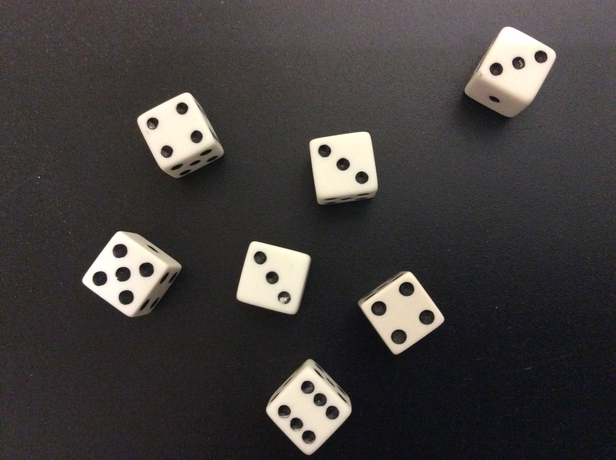
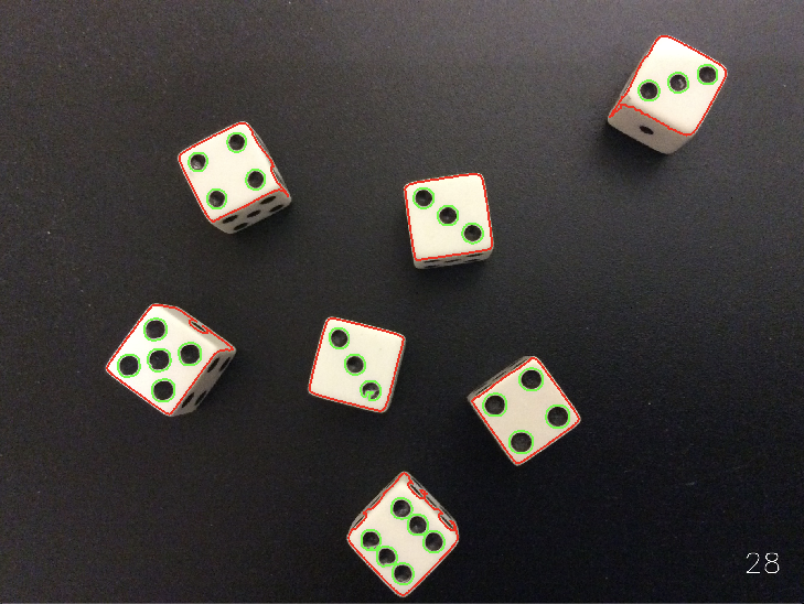
The functionality we have looked at here concentrates on external contours; but OpenCV's contour routine can find contours within contours (within contours...), resulting in a hierarchy of contours. With some careful programming you can, for example, write a program which processes an image of some dice to find all the spots on them and print their total:

The code to do the counting runs something like this:

contours, hierarchy = cv2.findContours (binary, cv2.RETR_TREE,
                                        cv2.CHAIN_APPROX_SIMPLE)
dice = []    # list of dice contours
spots = []   # list of spot contours

# Find dice contours.
for (i, c) in enumerate(hierarchy[0]):
    if c[3] == -1:
        dice.append (i)

# Find spot contours.
for (i, c) in enumerate(hierarchy[0]):
    if c[3] in dice:
        spots.append (i)

print ("Dice roll total:", len (spots))

I'm not suggesting you go ahead an implement this but it's useful to know that it is possible. In case you think you can build on this to automate the playing of dice games, you need to bear in mind that making the segmentation robust to lighting changes is very difficult!

All the laboratory scripts